Online Exhibition

Introduction

The KPG Online Exhibition presents practical examples of transparent and reproducible power-system analysis using the KPG Platform.

What This Exhibition Contains

The exhibition is organized around the three KPG modules:

• KPG TestGrid: synthetic Korean grid data for research and decarbonization studies

• KPG Run: optimization and simulation for ED, UC, DC-OPF, and AC-OPF

• KPG View: spatial visualization of networks and simulation outputs

Who This Is For

• Researchers and students learning power-system modeling

• Engineers and analysts building reproducible workflows

• Stakeholders evaluating practical open-grid applications

Showcase 1: System Behavior Snapshot

This showcase establishes the operating context used later in the LMP case.

1) Renewable Curtailment Context

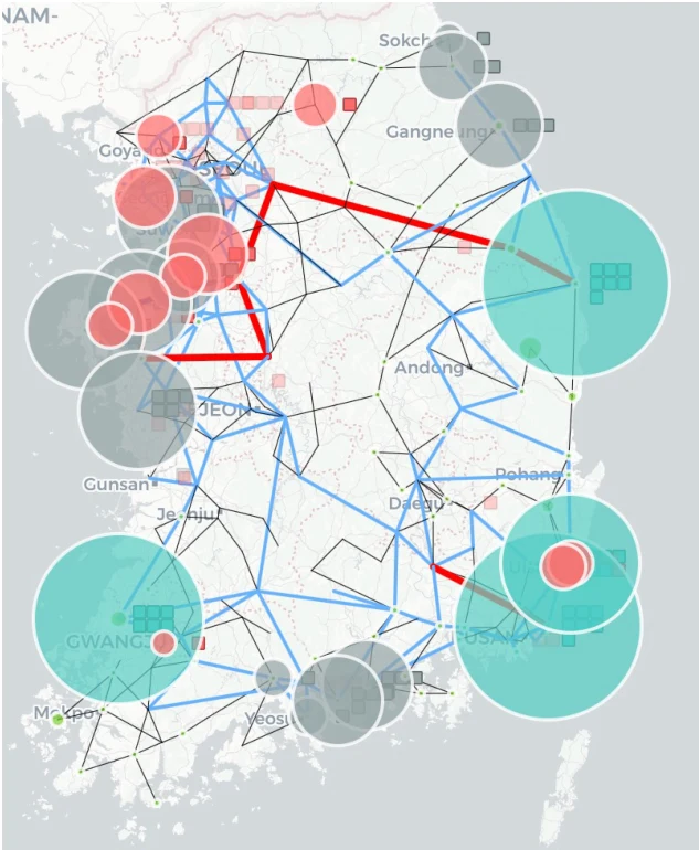
We start from a high-renewable operating condition where transfer limits can trigger curtailment risk in the Honam area.

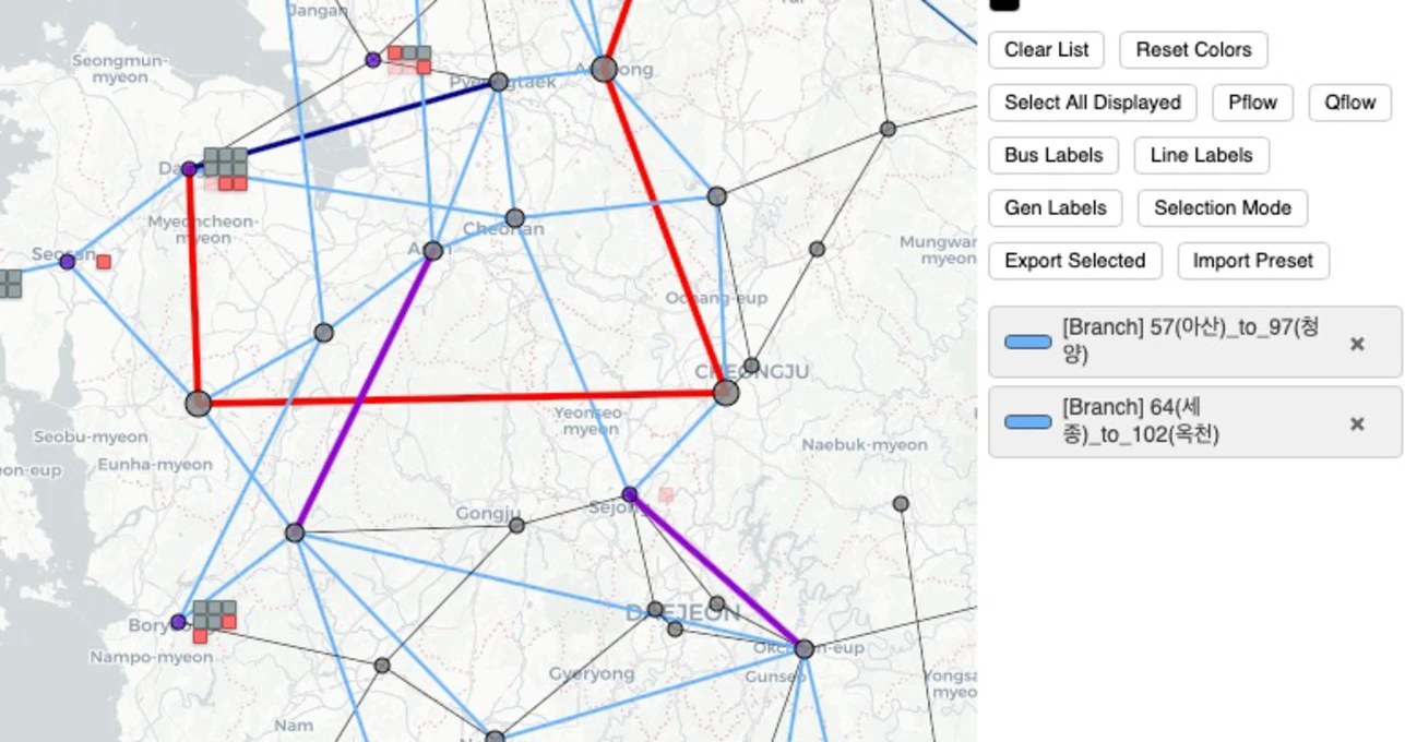
Honam-to-Chungcheong flowgate stability-limit context.

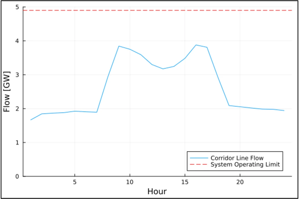
Flow result on the Honam-to-Chungcheong interface in KPG TestGrid.

The stability transfer limit of the Honam-to-Chungcheong flowgate is reported as 4.9 GW (Hooncheol Shin and Taeyong Song, “Analysis of the Impact of Solar Utilization on the Honam Power System,” 2024). To manage this limit, renewable generation in the Honam area is curtailed when northbound transfer stress becomes high.

KPG TestGrid is calibrated to 2022 conditions, so this limit is generally not reached even when renewable-driven northbound flow increases. However, as solar capacity expanded in 2023 and 2024, stability-related curtailment risk increased, and actual curtailment events have been observed since 2023.

2) Spring UC Behavior (Day 121)

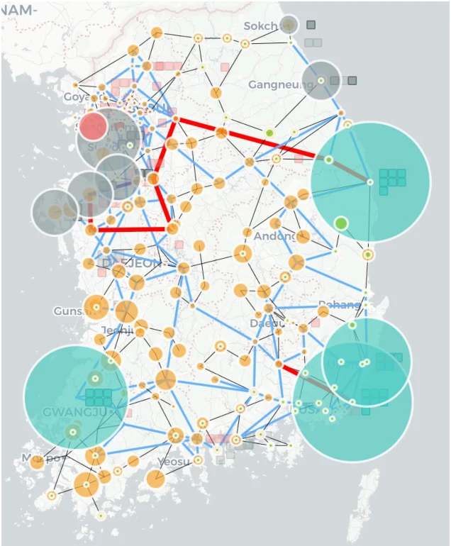
Under low-load and high-renewable conditions (Day 121), thermal dispatch reduces during midday and recovers in evening hours.

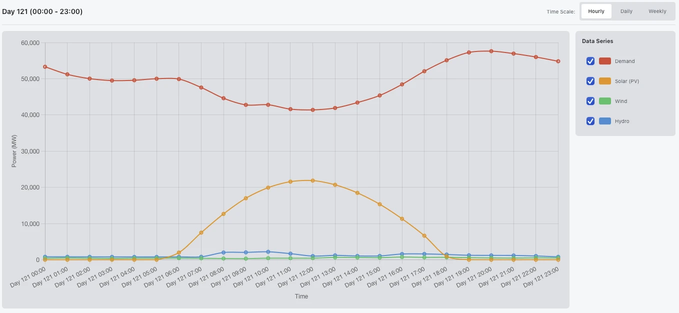
Representative spring-day profile (Day 121).

When system demand is low and solar generation is high, UC can decommit LNG units that normally serve peak demand.

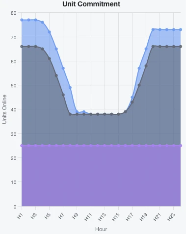
Day 121 UC dispatch result (hourly by resource).

Detailed snapshots (T=6, T=9, T=13, T=18) show this transition more concretely: as renewable output increases toward midday, LNG output is reduced or turned off, then restored as solar output declines.

Snapshot at `T=6`.

Snapshot at `T=9`.

Snapshot at `T=13`.

Snapshot at `T=18`.

Showcase 2: Locational Marginal Pricing (LMP)

Reproducible Codebase

• Main repository: KPG Platform LMP Repository

• Entry script: calculate_lmp.jl

• Core modules: src/Step4Lite.jl, src/runner.jl, src/network.jl, src/opf_math.jl

• Included dataset path: data/KPG193_ver1_5

• Main output pattern: outputs/ZonalResult_<output_name>_<day>_<hour>.csv

This section follows the public repository workflow and documents a runnable LMP case for KPG Platform users.

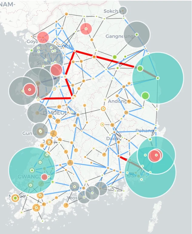
Why LMP Matters in This Case

Korean demand is heavily concentrated in the Seoul metropolitan area while a substantial share of generation is outside the region. This creates persistent transfer stress on key corridors, and nodal pricing is needed to explain location-specific marginal costs.

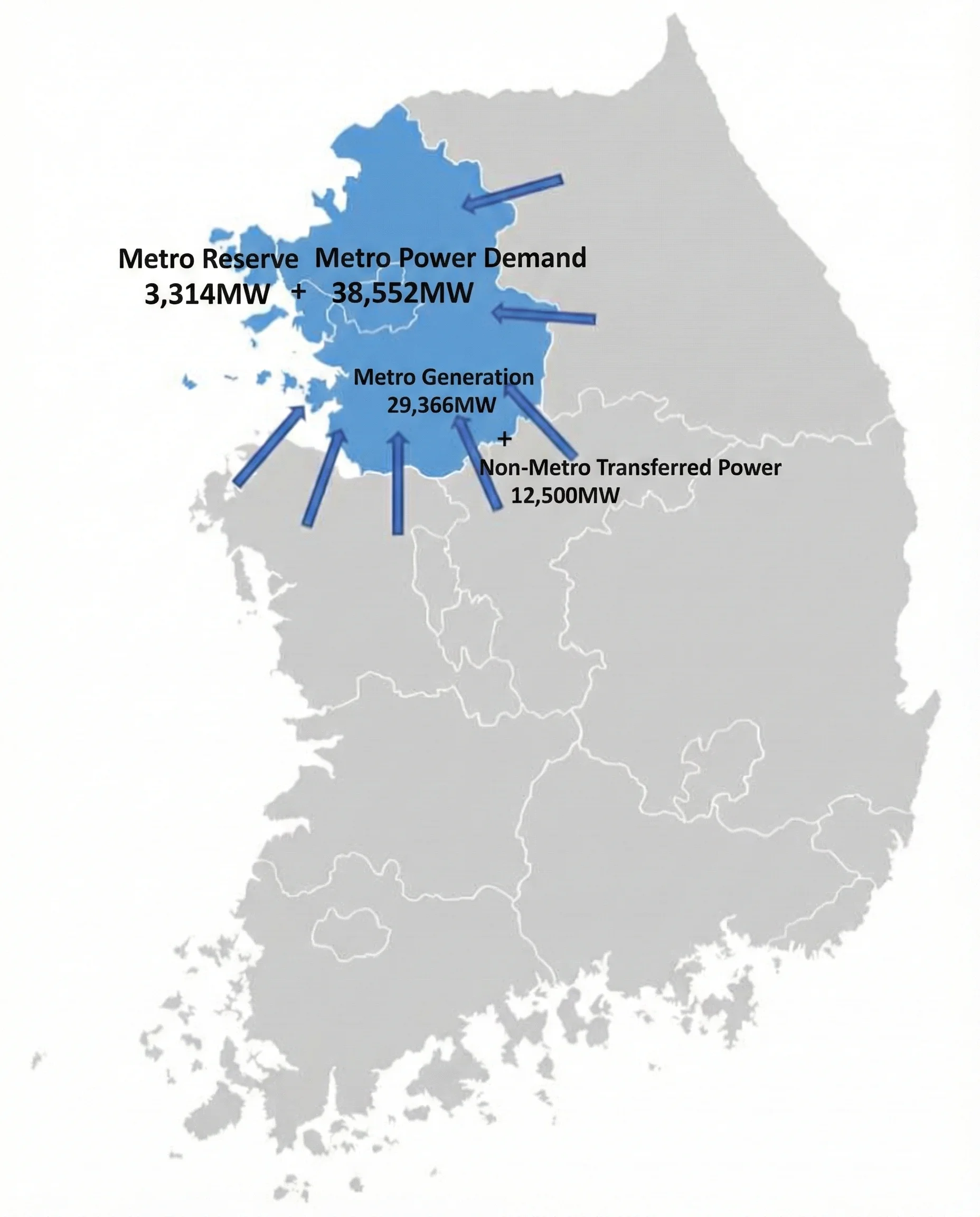
2023 Seoul Metropolitan Area supply and demand context.

LMP Definition and Decomposition

LMP at each bus is separated into energy, loss, and congestion components:

SMP is a single system-wide marginal value. LMP is node-specific and reflects network constraints directly, so regional price separation can be interpreted explicitly.

Reference: Detailed Explanation of SMP

Three-Stage Optimization in kpg-platform-lmp

• M0: solves commitment and reserve with flow constraints

• M1: updates loss model using loss-factor linearization based on M0

• M2: fixes commitment, re-solves dispatch, and computes final LMP decomposition from dual values

This M0 -> M1 -> M2 flow is implemented in src/runner.jl (run_step4) and is the exact workflow used for this exhibition.

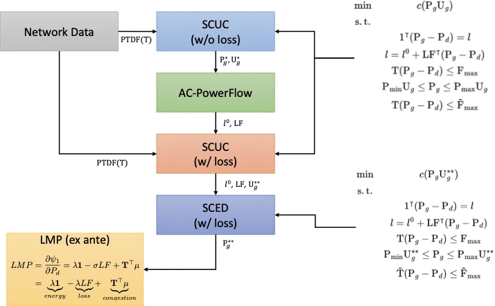
Day-ahead market stage and placement of the LMP case.

Default Case Configuration (from default_config)

• Time index: --day 188 --hour 18 (KST)

• Solver: Gurobi default, HiGHS supported

• HVDC transfer: bus-index 53 -> 51, 1.5 GW equivalent (15 pu, baseMVA 100)

• Reserve requirements: up 4.5 GW, down 1.2 GW

• Flowgate set (bindex pairs): (28,80), (38,84), (44,57), (47,60), (50,54), (50,62)

• Cost override input: input/kpg193_cost_lmp_backup.csv

• Network MAT input: data/KPG193_ver1_5/network/mat/KPG193_ver1_5_LMP.mat

Generator fuel-cost localization input used in this case (partial excerpt):

Run the Case (Reproduction)

# Clone using the repository URL in "Main repository" above.
git clone <kpg-platform-lmp-repository-url>
cd kpg-platform-lmp

julia -e 'using Pkg; Pkg.add(["CSV","DataFrames","JuMP","MAT","HiGHS"])'
julia calculate_lmp.jl --solver HiGHS --day 188 --hour 18

Advanced run example (same option names as repository README):

julia calculate_lmp.jl \
  --day 188 \
  --hour 18 \
  --solver HiGHS \
  --data-dir data/KPG193_ver1_5 \
  --mat-path data/KPG193_ver1_5/network/mat/KPG193_ver1_5_LMP.mat \
  --cost-path input/kpg193_cost_lmp_backup.csv \
  --output-dir outputs \
  --output-name upreserve_45_dnreserve_12_step4

Output Schema and Validation

The generated CSV includes:

• Bus

• LMP, LMP_E, LMP_L, LMP_C

• LMP_C_FLOWGATE

• latitude, longitude (joined from network/location/bus_location.csv)

Validation checks:

• Verify identity bus-by-bus: LMP = LMP_E + LMP_L + LMP_C

• Confirm output filename exists: outputs/ZonalResult_<output_name>_<day>_<hour>.csv

• Plot by latitude/longitude for a nodal map in KPG View or GIS tools

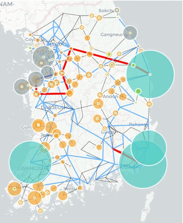
Reference Snapshot (Summer Peak, 18:00)

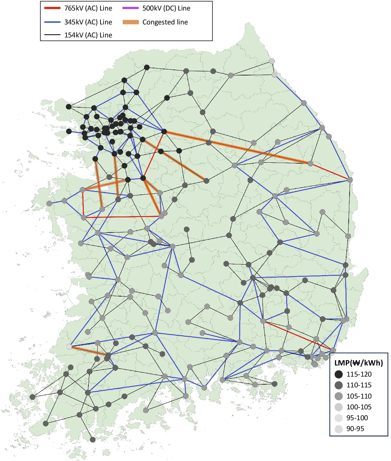
Summer-peak nodal LMP map (reference snapshot).

Replication Assets (Code + Data)

• LMP reproduction repository: KPG Platform LMP Repository

• Comparison/conversion repository: KPG Platform Converters Repository

• Base dataset repository: KPG TestGrid Repository