User Interface Guide
This guide explains the layout of the KPG Run interface and how to navigate the main panels and tabs.
Interface Layout
Main Components
1. Header Bar
- Application title
- Light, dark, and system (auto) themes selector
- Settings
- Current status indicator
2. Configuration Panel
- Data Source
- Problem Setup
- Solver
3. Main Workspace
- Editor
- Network Data
- Time Series
- Console
- Results
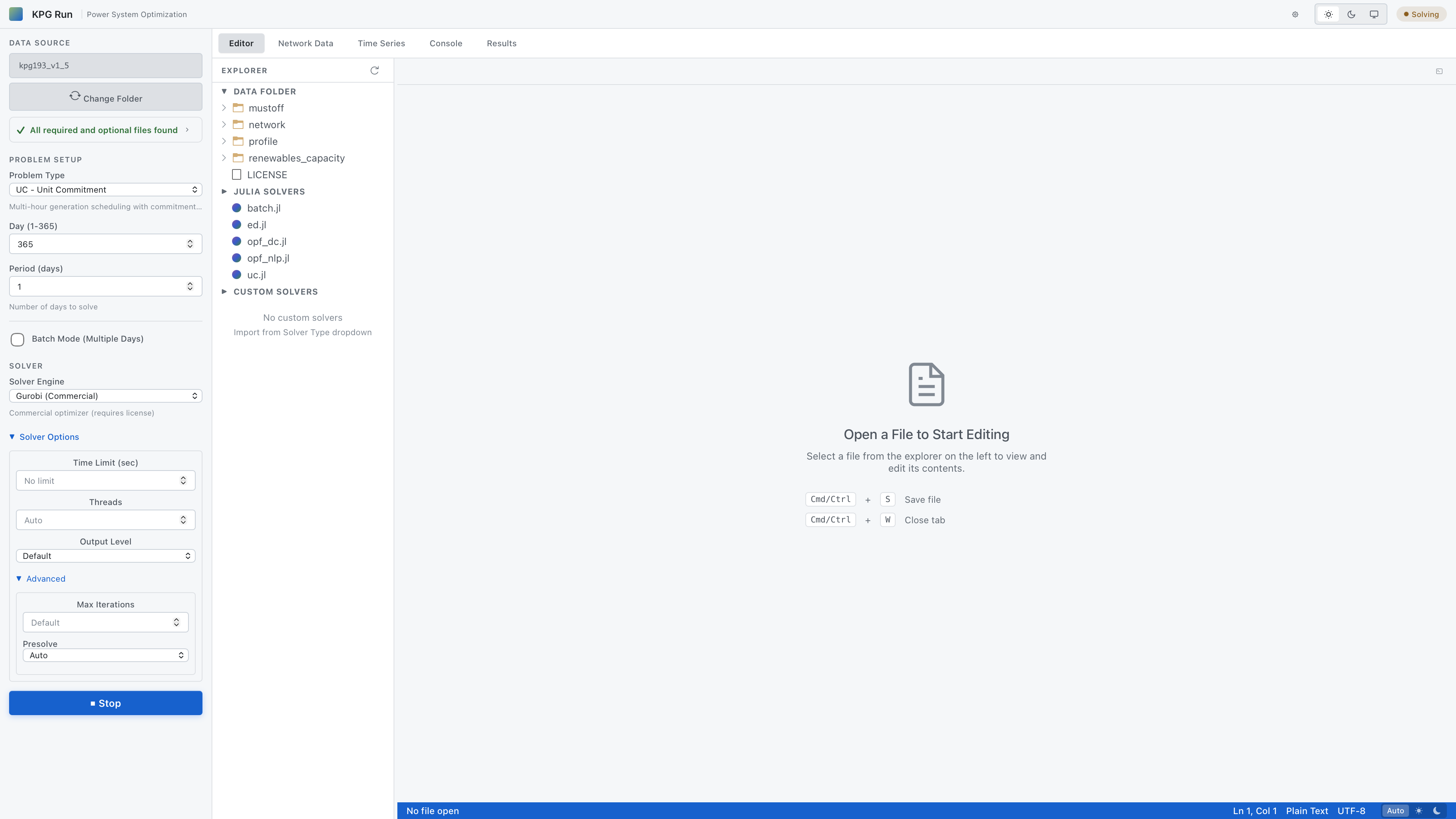
Configuration Panel
Use the Configuration panel to select the optimization model and define its basic settings.
Data Source
- Select a test system folder to use as the data source for the run.
- The Change Folder button opens a file dialog to choose a folder.
- The Data validation checker verifies that required and optional files are present in the selected folder. (Expandable)
Problem Setup
Problem Type:
- ED: Economic Dispatch (simplest)
- UC: Unit Commitment (temporal)
- DC-OPF: DC Optimal Power Flow (network)
- AC-OPF: AC Optimal Power Flow (most complex)
- Custom Solver: User-defined model
Problem Settings:
- Day (1-365): Selects the day of year for which to run the optimization.
- Batch Mode (Multiple Days): Enables solving across multiple consecutive days when supported. (Planned)
- Period (days): Sets the number of consecutive days to include in the optimization horizon. (UC only)
Solver
Solver Engine
- Solver-specific options: Additional fields may appear depending on the chosen problem type and solver engine (for example, maximum iterations and print level for AC OPF).
- Solve button starts the optimization with the current configuration.
Solver Options
- Time Limit (sec): A maximum time limit for the solver to run.
- Threads: Number of CPU threads to allocate to the solver. (UC only)
- Output Level: Verbosity of solver output in the console.
- Advanced Options:
- Max Iterations: Maximum number of iterations before termination.
- Presolve: Enable or disable presolve routines. (UC only)
Buttons
Solve Button
- Starts optimization
- Disabled during solving
- Changes to Stop when running
Stop Button
- Appears during solving
- Terminates solver
Editor Tab
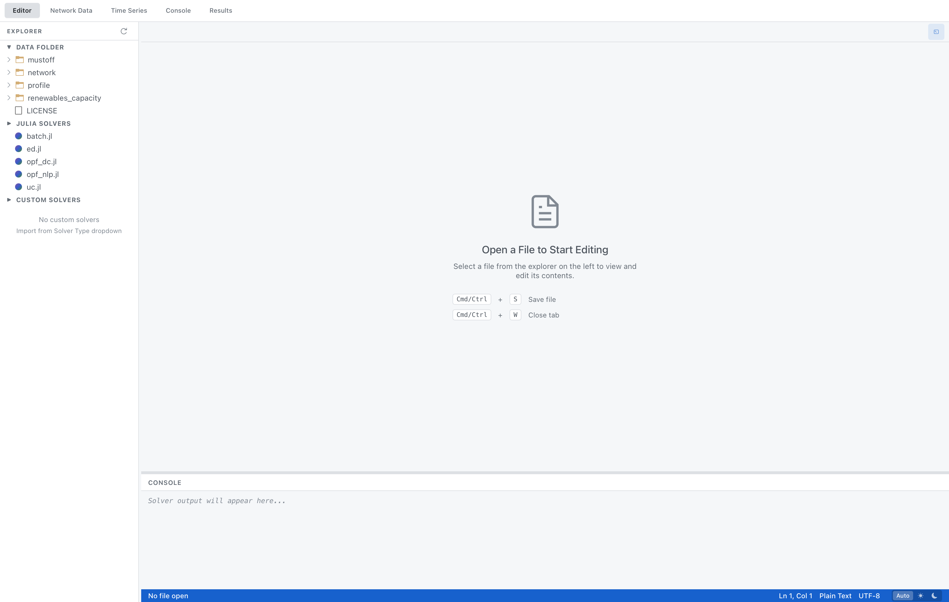
When the Editor tab is active:
- File Explorer (left pane)
- Displays the loaded Data Folder (e.g.,
network,profile,renewables_capacity) and available Julia Solvers (ed.jl,opf_dc.jl,uc.jl, etc.). - Selecting a file from the explorer opens it in the editor pane.
- Displays the loaded Data Folder (e.g.,
- Editor Pane (center)
- Shows the contents of the currently selected file.
- Supports standard editing operations and keyboard shortcuts (e.g., Cmd/Ctrl + S to save, Cmd/Ctrl + W to close the current tab).
- Multiple files can be opened simultaneously, each in its own tab.
- File Path Bar (bottom)
- Shows the path of the file currently open in the editor.
- Console Panel
- Displays real-time output from the solver when an optimization is running.
- Can be toggled using Cmd/Ctrl + J or the button in the upper-right corner.
Network Data Tab
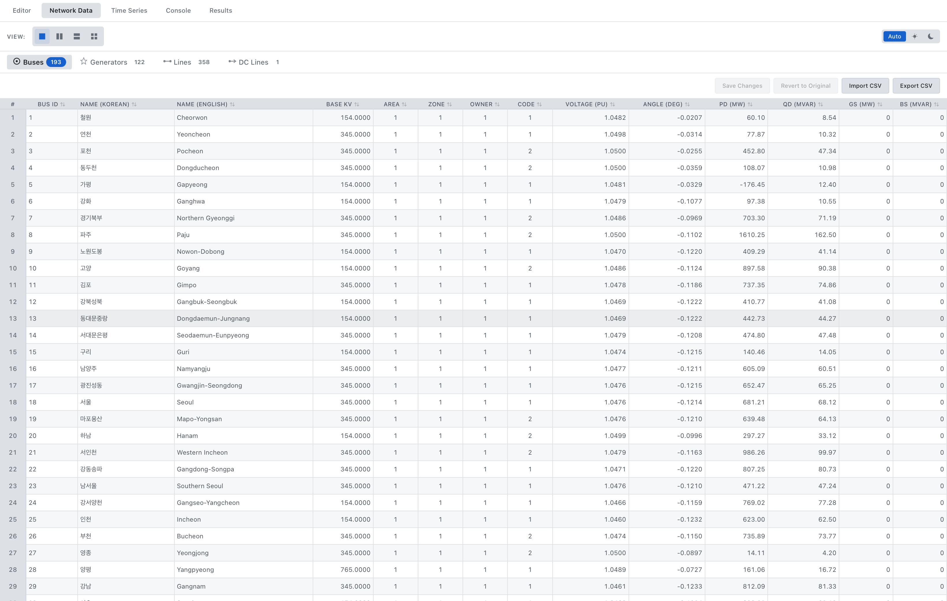
The Network Data tab provides a structured view of the input data for the selected test system. It is used to inspect and edit buses, generators, transmission lines, and DC lines before running an optimization.
- View selector controls how network data are displayed
- Single view (1x1)
- Two columns (1x2)
- Two rows (2x1)
- Grid (2x2)
- Object tabs switch between Buses, Generators, Lines, and DC Lines. Each tab label shows the number of records currently loaded (for example, Buses 193).
- Data table displays the fields for the selected object type (such as BUS ID, NAME, etc.). Cells can be edited directly to modify network parameters.
Editing and file operations
The values in this table are editable. When a cell is modified, the change is highlighted in yellow. You can either apply the pending edits to the network data or revert them to their original values. Network data can also be imported from, or exported to, CSV files.
- Save Changes applies the edits in the table to the currently loaded network data.
- Revert to Original discards unsaved edits and restores the data to the state loaded from the test system folder.
- Import CSV replaces the current table with data loaded from a CSV file that matches the expected schema.
- Export CSV writes the current table contents to a CSV file for external analysis or version control.
Time Series Tab
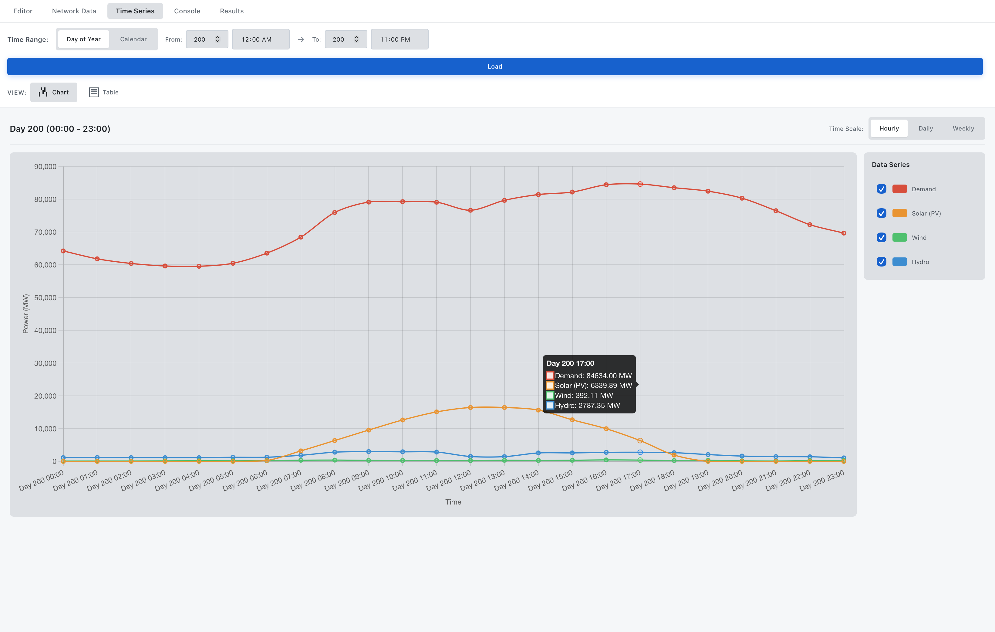
The Time Series tab provides an overview of load and renewable generation profiles used by the selected test system. It allows you to inspect how demand and resource availability evolve over time before running an optimization.
Time Range Controls
- Time Range mode lets you choose whether to select data by Day of Year or by Calendar date.
- From / To specify the start and end date/time for the time window.
- The Load button applies the selected time range and reloads the chart and table.
View Modes
- Chart displays a time-series line chart of the selected data series (e.g., Demand, Solar, Wind, Hydro).
- Table shows the same data in tabular form for precise inspection or export.
Chart Interactions
- Tooltips appear when your cursor hovers over the chart, showing the value for each active series.
- Time Scale switches between Hourly, Daily, and Weekly aggregation.
- Data Series panel toggle individual series (Demand, Solar, Wind, Hydro) on or off to focus on specific resources.
Console
Solver Output
- Displays the raw log output from the currently running or most recent optimization (for example, Gurobi progress, convergence information, and final status).
- Messages are streamed in real time while a solve is in progress.
- Use Clear to remove the current log contents and prepare for a new run.
Julia REPL
- Provides a Julia prompt inside KPG Run, where you can enter Julia code.
- Use the Restart button to reset the REPL session, or the Clear button to clear the visible output without restarting the process.
The text field at the bottom of the view is the input line; press Enter to execute the current command.
Results Tab
After an optimization run finishes, results are displayed in the Results tab. Here, you can review the problem configuration, solution status, objective value, and other summary information. The available sub-tabs depend on the selected solver and provide detailed views of the corresponding results.
All models return the active power dispatch after solving.
For OPF models that include network constraints, line flows and bus angles are reported. Among the four built-in models, only the AC-OPF, which considers the AC network, provides bus voltage magnitudes and reactive power (Q) outputs. Unit commitment schedules are available only for the UC model.
For more information on these model differences, refer to the Formulation section.
To save results, use the Save to Folder or Download ZIP buttons. These actions export the results in CSV, JSON, and GeoJSON formats to a user-selected location.
Summary View:
- Solved problem
- Test system
- Day
- Solution status
- Objective value
Detailed Results
Tabs within Results:
- Dispatch Table
- Network Flows (DC/AC-OPF only)
- Commitment Schedule (UC only)
Dispatch Table View
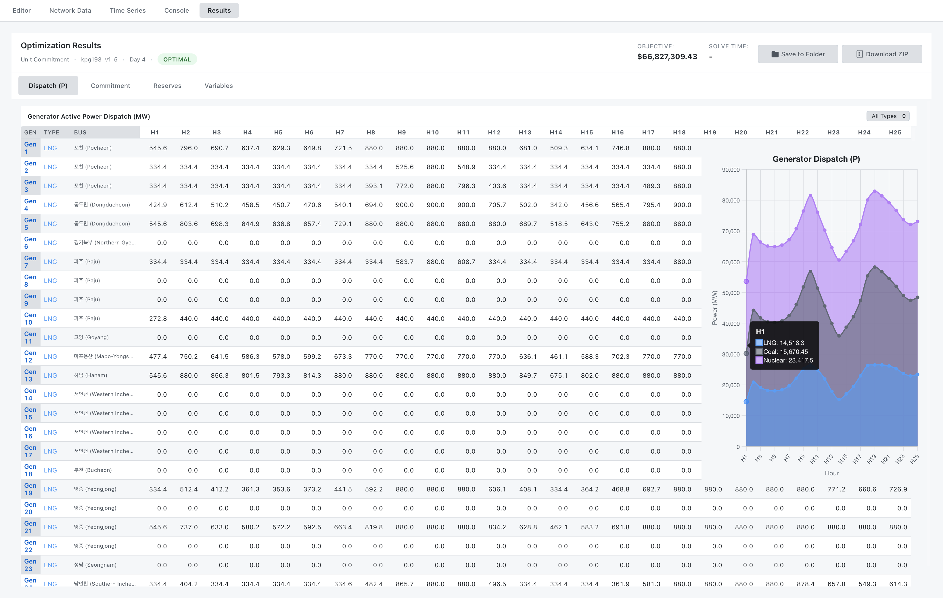
Table Columns:
- Gen: Identifier of each generator.
- Type: Fuel type of the generator.
- Bus: Bus name to which the generator is connected.
- H1–H24: Time periods included in the analysis.
Features:
- Generator Dispatch plot displays a stacked time-series of power dispatch by fuel type over all hours.
- Tooltips appear when your cursor hovers over the plot, displaying the hour and the dispatched power for each fuel type.
- Fuel-type filter limits the table to selected fuel types.
Network Flows View (OPF Only)
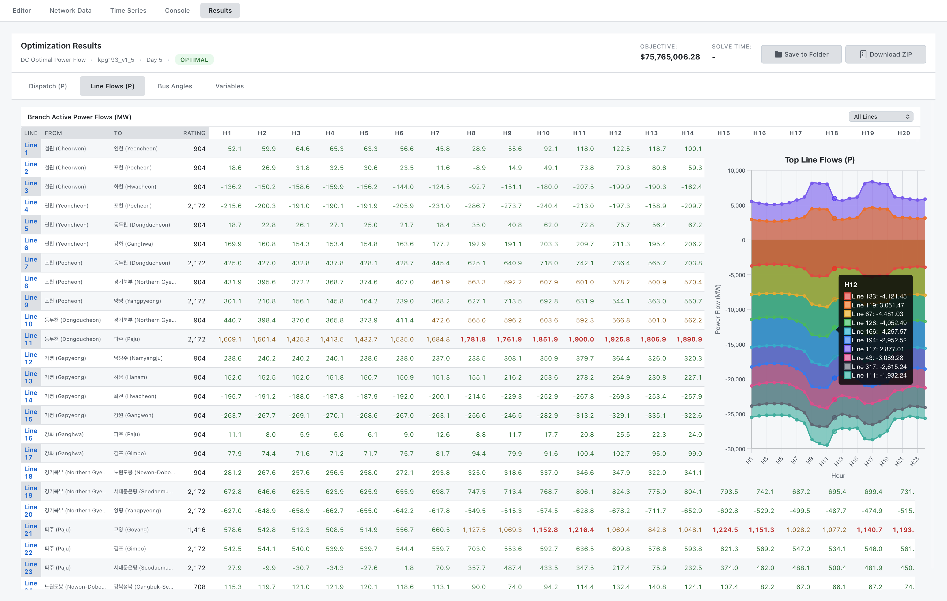
Optimal Power Flow (OPF) solves the optimization problem on a network model and computes power flows on each transmission line. This allows operators to identify which lines are congested. When the flow on a line exceeds its rating, corrective actions are required to relieve the overload.
In KPG Run, the Line Flows tab provides a spreadsheet and a time-series plot showing how power flows evolve over time for each line.
Table Columns:
- Line: Identifier of each transmission line.
- From / To: Sending and receiving buses for each line.
- Rating: Flow limit (thermal rating) of the line.
- H1–H24: Time periods included in the analysis.
Features:
- Top Line Flows plot shows a stacked time-series of power flows for the highest flowing lines over all hours.
- Tooltips appear when your cursor hovers over the plot, showing the hour and power flow for each displayed line at each hour.
- Line-loading filter filters the table by line-loading category:
- All Lines
- Lines whose loading never exceeds 50% at any hour
- Lines whose loading exceeds 80% at least once
- All remaining lines (with loading between 50% and 80%)
Line Loading (% of rating):
- 🔴 Congested (80-100%)
- 🟡 Heavily loaded (50-80%)
- 🟢 Normal (0-50%)
Commitment Schedule (UC Only)
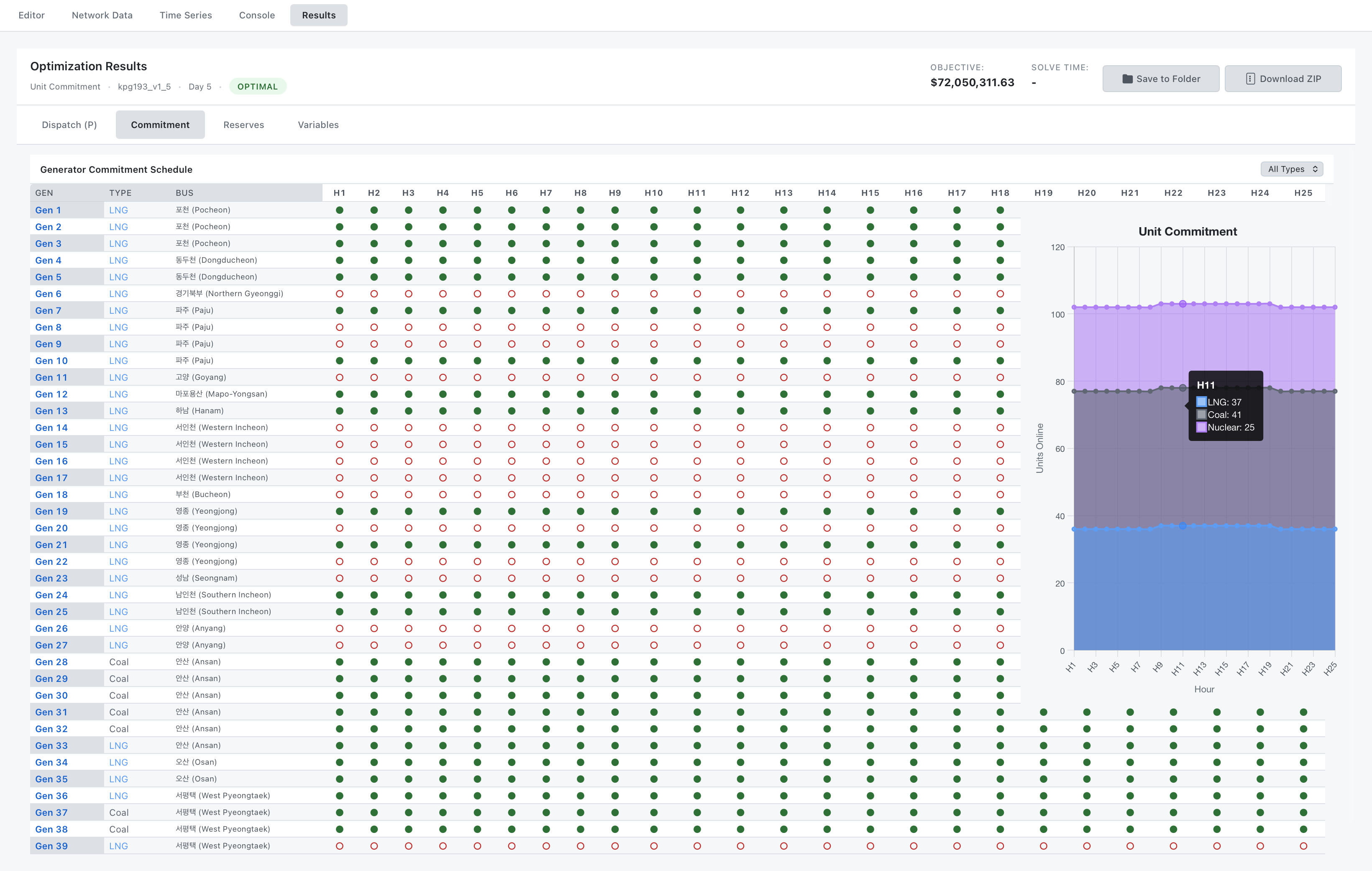
Table Columns:
- Gen: Identifier of each generator.
- Type: Fuel type of the generator.
- Bus: Bus name where the generator is connected.
- H1–H24: Time periods included in the analysis.
Features:
- Commitment markers show the on/off status of each generator for every time period.
- Tooltips appear when your cursor hovers over the plot, showing the number of online units by fuel type at each hour.
- Fuel-type filter limits the table to selected fuel types.
Parameter Guide
Day Selection
Input: Day number (1-365)
| Input | Description |
|---|---|
1 | January 1 |
15 | Mid-January (mid-winter) |
75 | Mid-March (spring) |
200 | Mid-July (mid-summer) |
290 | Mid-October (fall) |
365 | December 31 |
Validation:
- Red border if invalid (< 1 or > 365)
- Tooltip shows valid range
Hour Description
Critical hours:
| Hour | Time | Typical Usage |
|---|---|---|
| 3 | 2-3 AM | Minimum load |
| 12 | 11 AM-12 PM | Midday, peak solar |
| 14 | 1-2 PM | Peak load (summer) |
| 18 | 5-6 PM | Evening peak |
| 20 | 7-8 PM | Winter evening peak |
Results Export
Export Buttons
Both buttons open a dialog to select a directory where the results will be saved.
- Save to Folder:
- Saves result files (CSV, JSON, GeoJSON) to the chosen folder.
- Download ZIP:
- Creates a ZIP archive of all result files.
Export Formats
CSV (Tabular data):
A CSV (Comma-Separated Values) file is a plain-text tabular format where each line is a row and fields are separated by a delimiter (typically a comma).
KPG Run exports result data in CSV format. For each model, results are stored in CSV files with a predefined structure.
Features:
- Buses
- Generators
- Branches
- DC lines
JSON (Structured data):
The JSON format contains a basic summary of the simulation results and the structure of the result files. The format is as follows:
{ "snapshots": [ { "hour": 1, "filename": "geojson/snapshot_t01.geojson", "index": 1, }, ... { "hour": 24, "filename": "geojson/snapshot_t24.geojson", "index": 24, } ], "files": { "generators": "generators_timeseries.csv", "branches": "branches_timeseries.csv", "dclines": "dclines_timeseries.csv", "buses": "buses_timeseries.csv", }, "simulation": { "start_time": "2025-12-16T14:30:00", "day": "200", ... "type": "UC", "system": "KPG193" }}GeoJSON (For KPG View):
Optimization results are stored in GeoJSON format for visualization in KPG View. For each time snapshot, the file contains location and information for buses, generators, and branches, as well as ratings, optimization outputs, feature group information, and some summary values.
{ "features": [ { "geometry": { "coordinates": [ Longitude, Latitude ], "type": "Point" }, "id": "Bus_1", "properties": { "num_buses": 1, ... "Hydro_Pmax":0.0 }, "type": "Feature" }, ... } ] }, "type": "FeatureCollection",}Next Steps
- Try your first optimization: Getting Started →
- Understand the math: Formulations →
- See complete examples: Workflows →
- Visualize results: KPG View →